Visualization
mGrowthCtrl provides plotting utilities for visualizing experimental data, model fits (see Least-Squares Fitting), and MCMC results (see MCMC Fitting). To experiment with the visualization settings, we recommend exploring the jupyter notebooks in the “examples” directory.
Plotting Data with Model Overlay
- mgrowthctrl.utils.plot.plot_data_with_overlay(
- df: DataFrame,
- sim=None,
- mcmc_sims=None,
- overlay: Literal['splines', 'model', 'both'] | None = 'splines',
- time_col: str | None = None,
- x_cols: Sequence[str] | None = None,
- s_cols: Sequence[str] | None = None,
- x_err_cols: Sequence[str] | None = None,
- s_err_cols: Sequence[str] | None = None,
- n_spline_points: int = 400,
- shade_percentiles: bool = False,
- percentiles: Tuple[float, float] = (2.5, 97.5),
- thin_alpha: float = 0.25,
- thin_lw: float = 0.75,
- thick_lw: float = 2.5,
- title: str | None = None,
- save_prefix: str | None = None,
- **kwargs,
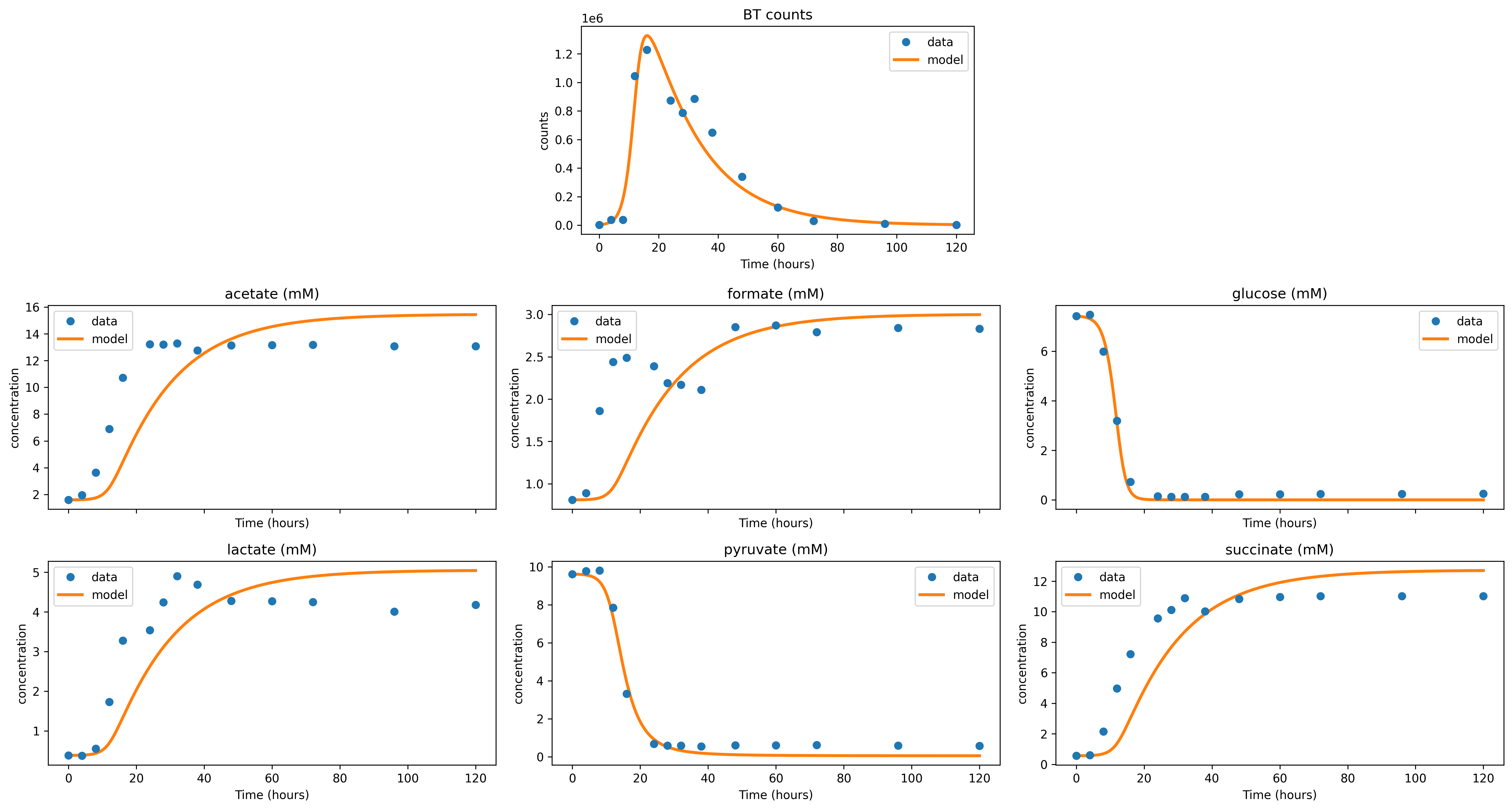
Plot the data in the given dataframe, interpreting certain columns as species (X), metabolites (S), or time. If given a simulation, can plot it along with the data.
- Parameters:
df – The input dataframe used for fitting the model
sim – A predicted simulation to plot along with the data. Should be a dictionary or a
SimpleNamespaceobject that is produced by one of thepredictorsimulatemethods in the package.mcmc_sims – A set of MCMC simulations to visualize
overlay – Whether to draw the model simulation and, additionally, whether to connect the given datapoints with splines.
time_col – The name of the time column in the data
x_cols – The names of species (X) columns
s_cols – The names of metabolite (S) columns
x_err_cols – The names of species (X) error columns
s_err_cols – The names of metabolite (S) error columns
n_spline_points – Number of points to generate for the spline visualization
shade_percentiles – Whether to add colored shading to percentile bands
percentiles – What range of percentiles to shade
thin_alpha – Transparency of thin lines used to represent uncertainty
thin_lw – Line width of thin lines used to represent uncertainty
thick_lw – Line width of thick lines for splines and model simulation
title – Title of the chart
save_prefix – If given, will save images as filenames with the given prefix
Example output for a model fitted with least-squares:
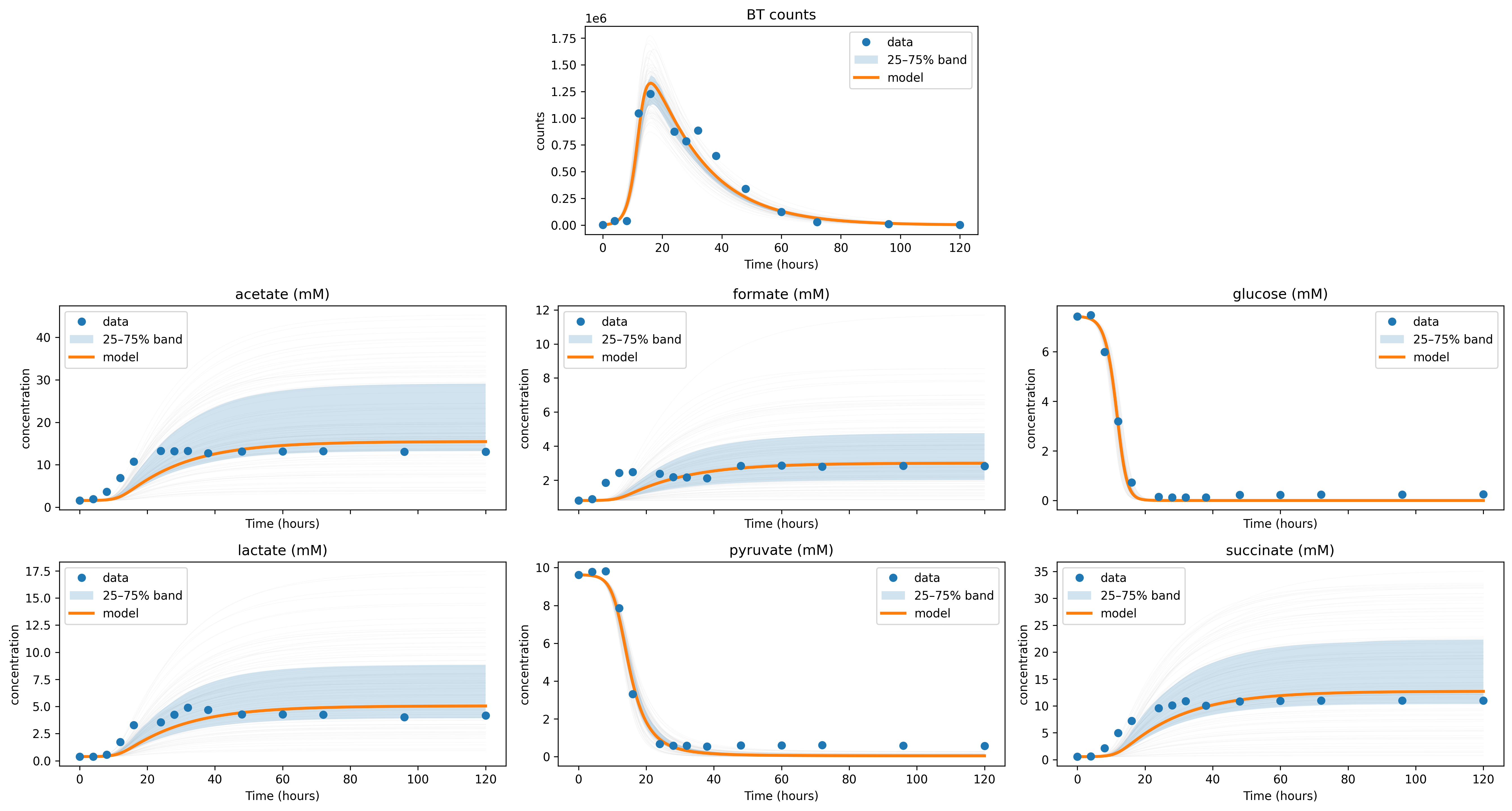
Example output for an MCMC fit, including error bands:
MCMC Diagnostics
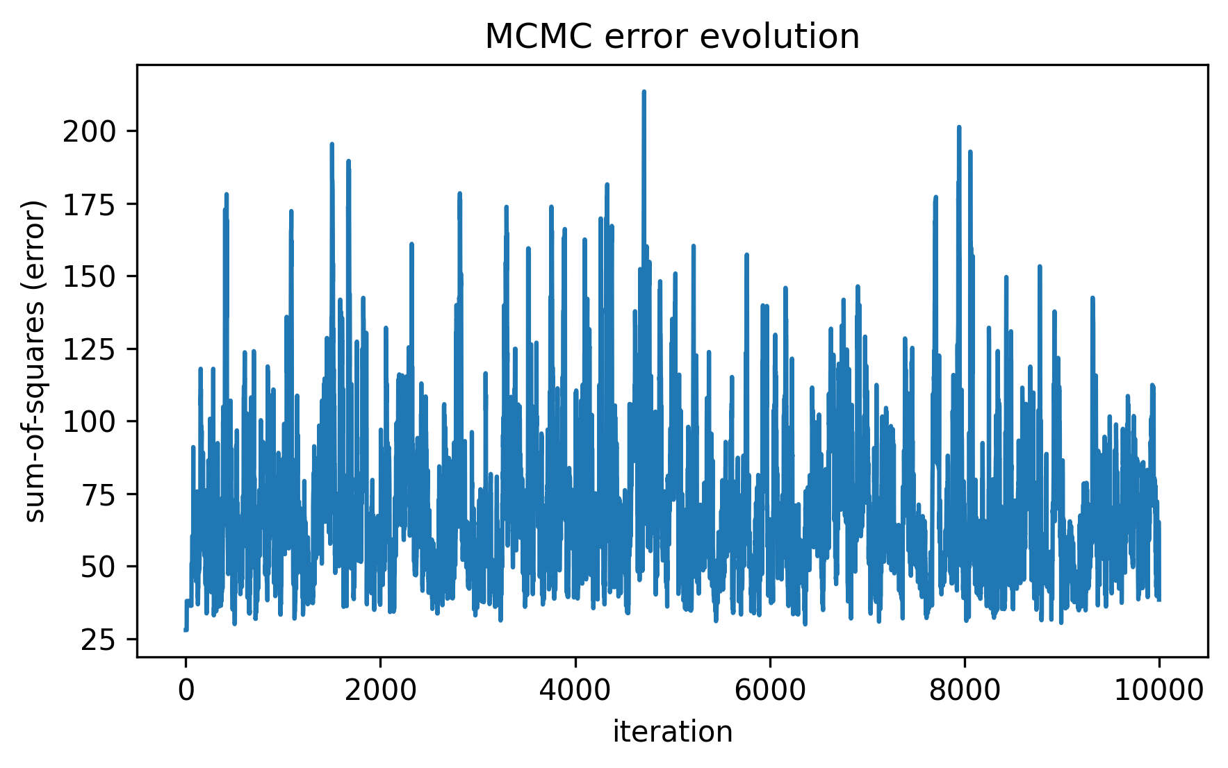
- mgrowthctrl.utils.plot.plot_mcmc_error_evolution(sschain, save_prefix=None)
Plot a visualization of the sum-of-squares error chain produced as the result of a MCMC fitting process.
- Parameters:
sschain – The chain object generated by MCMC functions in the package
save_prefix – If given, will save images as filenames with the given prefix
Example output:
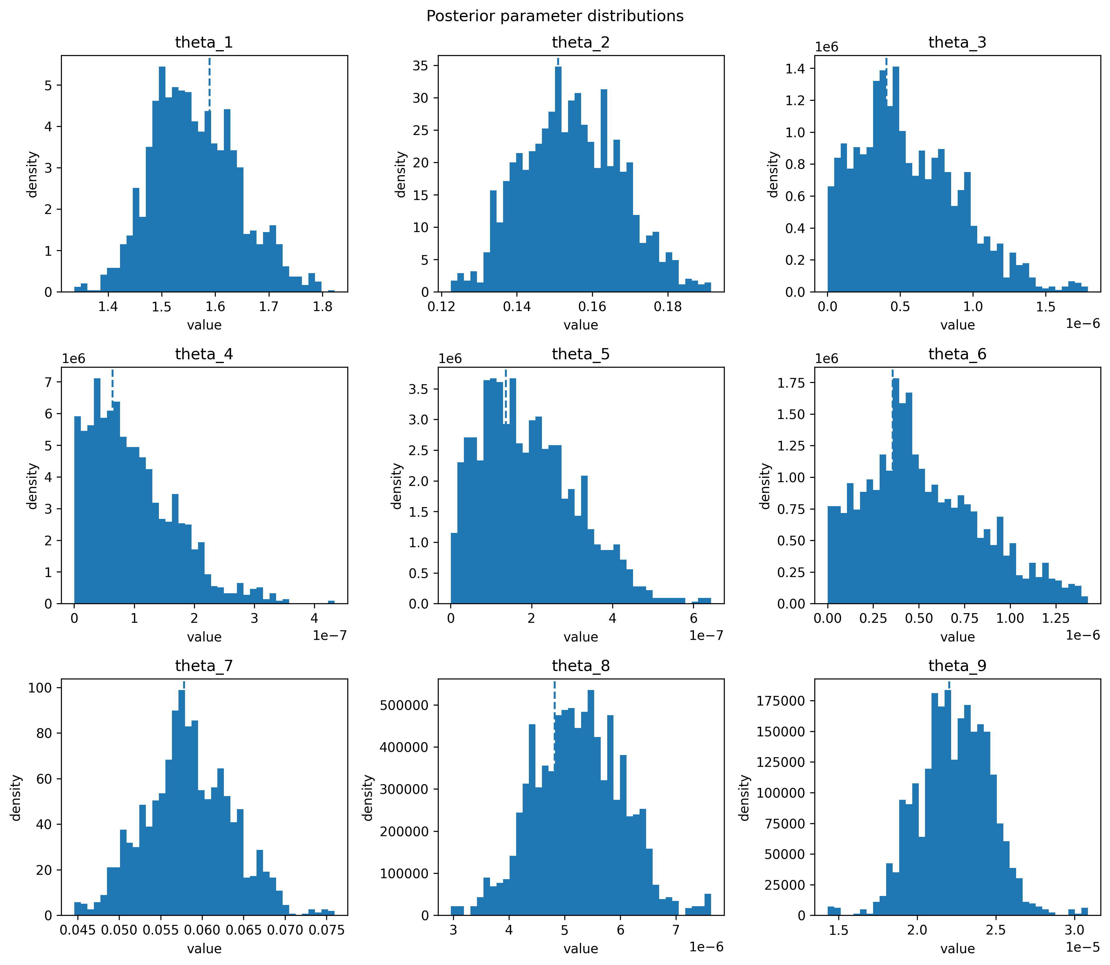
- mgrowthctrl.utils.plot.plot_parameter_distributions(
- post,
- theta_mle: Sequence[float] | None = None,
- names: Sequence[str] | None = None,
- bins=40,
- save_prefix=None,
Plot the posterior parameter distributions found by the MCMC fitting process as histograms.
- Parameters:
post – Posterior parameter distribution, as generated from the fitting functions in the package.
theta_mle – A list of maximum likelihood estimates of the parameters
names – The names of the plotted parameters
bins – Number of bins to use for the histograms
save_prefix – If given, will save images as filenames with the given prefix
Example output: