Get Started

This guide walks you through the basic workflow of loading data, fitting a consumer–resource model (CRM), and visualizing the results. For installation instructions, see the Installation section.

Loading Data

Load experimental time-series data from a CSV file:

from mgrowthctrl.utils.data import Dataloader

data = Dataloader()
data.load_local_data(
    "examples/datasets/BT_WC_export.csv",
    x_selector=r"BT counts",
)

This example uses the dataset BT_WC_export.csv. For further details on the data loader, see the Data Loading section.

Initializing and Fitting a Model

We can create a CRM with default parameters and fit it by using least-squares fitting:

from mgrowthctrl.models import CRModel, CRModelParams

# Initialize parameters
params = CRModelParams.from_shapes(n=len(data.X_names), m=len(data.S_names))

# Create model
model = CRModel(names=data.names, params=params)
print(model.n, model.m)

# Fit model with the defaults (updates internal parameters)
model.fit(
    df=data.df,
    time_col=data.time_col,
    x_cols=data.X_names,
    s_cols=data.S_names,
)

If we use this model, it’s likely that the fit won’t be very good, because we don’t have reasonable default parameters. In this particular example, since we only have data for a single species, we can extract a good guess for them from the data:

from mgrowthctrl.models import CRModel, CRModelParams

# Initialize model with parameters from the data
model = CRModel.from_single_species_data(
    df=data.df,
    time_col=data.time_col,
    x_col=data.X_names[0],  # Note: expects a single species string here
    s_cols=data.S_names,
)

model.fit(
    df=data.df,
    time_col=data.time_col,
    x_cols=data.X_names,
    s_cols=data.S_names,
)

We’ll use this second example for the next sections, since it will provide better predictions. Note that the CRModel.from_single_species_data() method is only usable here because we have a monoculture.

If you have a culture with multiple species, you should go through the Consumer-Resource Model tutorial, where you can find a discussion of the parameters along with the full reference documentation of the CRModelParams class.

Simulating Trajectories

Generate model predictions:

import numpy as np

# Time points
t_sim = np.linspace(data.start_time, data.end_time, num=200)

# Simulate
sim = model.simulate(data.y0, t_sim)

print(sim.t.shape)
print(sim.X.shape)
print(sim.S.shape)

Visualization

Plot data with model overlay using plot_data_with_overlay():

from mgrowthctrl.utils.plot import plot_data_with_overlay

plot_data_with_overlay(
    data.df,
    sim=sim,
    overlay="model",

    # Column names:
    time_col=data.time_col,
    x_cols=data.X_names,
    s_cols=data.S_names,

    # If save prefix is provided, saves plots to files:
    # - example_plot_species.png
    # - example_plot_metabolites.png
    save_prefix="example_plot",
)

Here’s what those predictions look like:

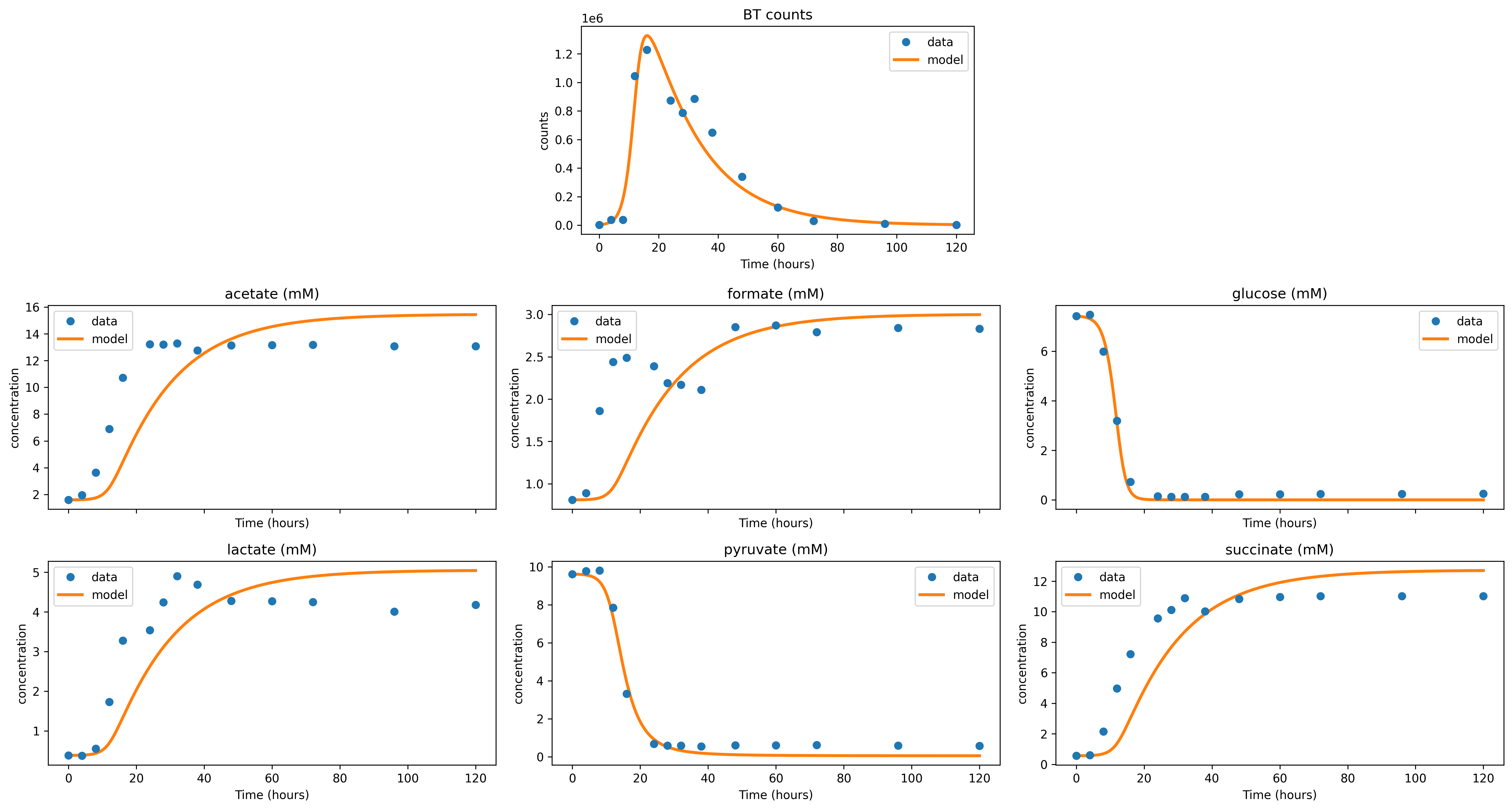
Further visualization options are described in the Visualization section.

If you’d like to save the simulation data in a CSV file for later plotting or analysis, you can use the utility function save_simulation_results():

from mgrowthctrl.utils.save import save_simulation_results

save_simulation_results(sim, data.names, 'saved_data.csv')