Simulating Consumer-Resource Dynamics

This tutorial builds on the Get Started example and explains in more detail how to set up a simple Consumer-Resource Model (CRM), simulate it, and fit it to data.

Loading Data

As in the Get Started example, we load experimental time-series data from the BT_WC_export.csv file:

from mgrowthctrl.utils.data import Dataloader

data = Dataloader()
data.load_local_data(
    "examples/datasets/BT_WC_export.csv",
    x_selector=r"BT counts",
)

For further details on the data loader, see the Data Loading section.

Initializing, Fitting, and Visualizing a CRM

We first create and fit a CRM to reproduce the output from the Get Started example:

import numpy as np
from mgrowthctrl.models.crm.model import CRModel, CRModelParams
from mgrowthctrl.utils.plot import plot_data_with_overlay

# Initialize parameters
params = CRModelParams.from_shapes(n=len(data.X_names), m=len(data.S_names))

# Create model
model = CRModel(names=data.names, params=params)
print(model.n, model.m)

# Initialize model with parameters from the data
model = CRModel.from_single_species_data(
    df=data.df,
    time_col=data.time_col,
    x_col=data.X_names[0],  # Note: expects a single species string here
    s_cols=data.S_names,
)

model.fit(
    df=data.df,
    time_col=data.time_col,
    x_cols=data.X_names,
    s_cols=data.S_names,
)

# Time points for simulation
t_sim = np.linspace(data.start_time, data_end_time, num=200)

# Simulate
sim = model.simulate(data.y0, t_sim)

# Visualization
plot_data_with_overlay(
    data.df,
    sim=sim,
    overlay="model",

    # Column names:
    time_col=data.time_col,
    x_cols=data.X_names,
    s_cols=data.S_names,

    # If save prefix is provided, saves plots to files:
    # - example_plot_species.png
    # - example_plot_metabolites.png
    save_prefix="example_plot",
)

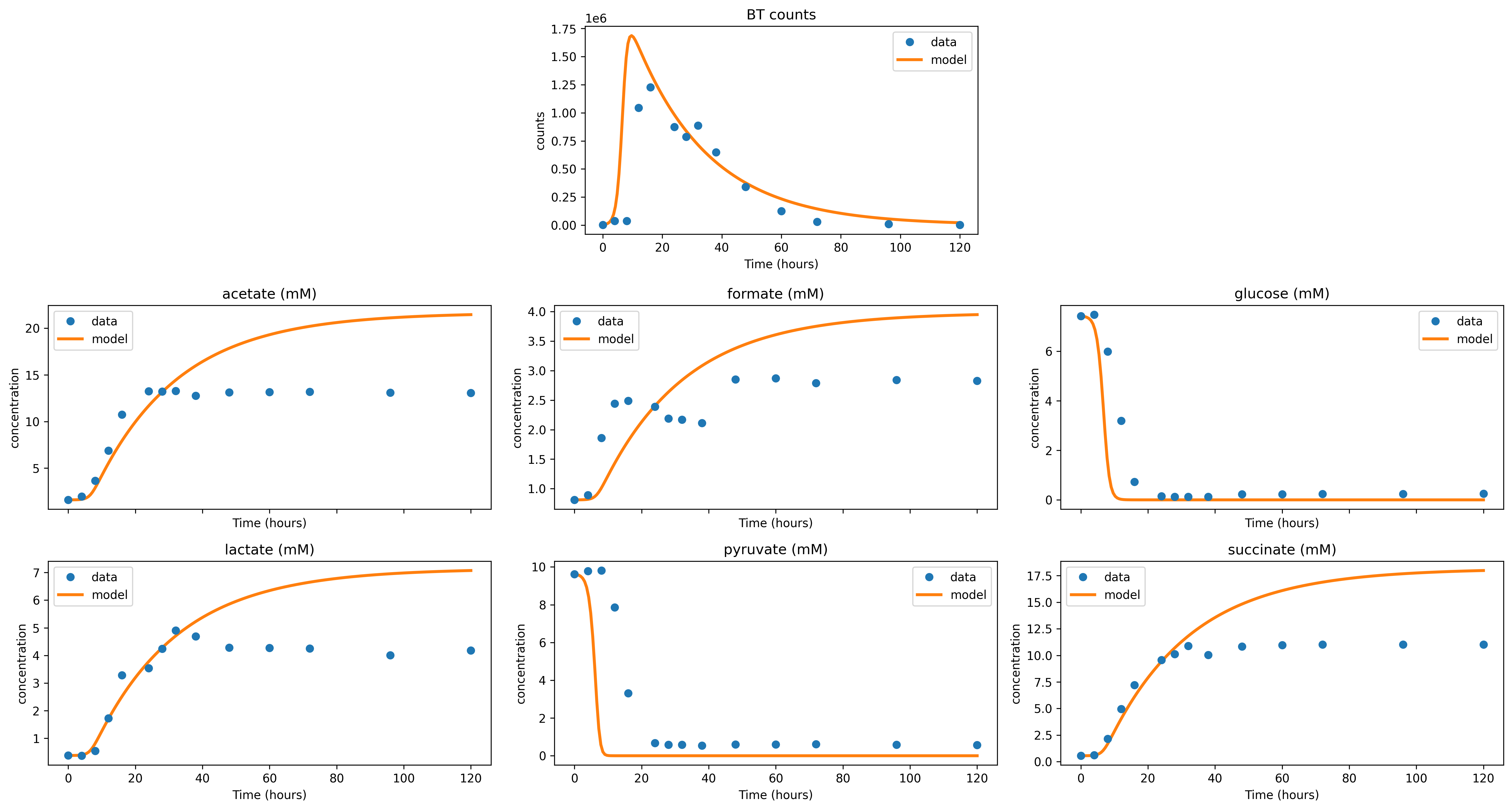
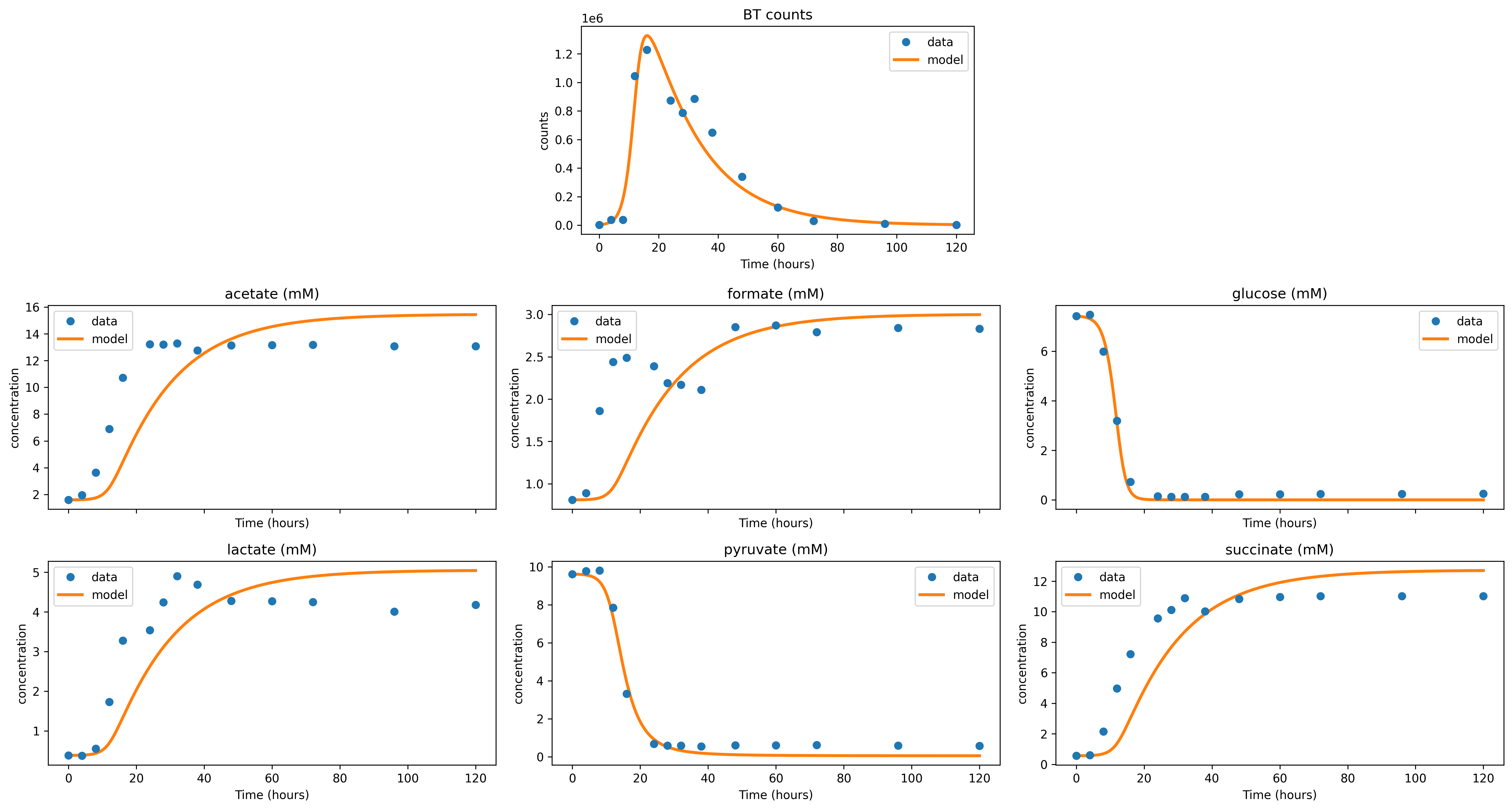
The CRModel.from_single_species_data() function initializes growth, uptake, and production parameters using mechanistic information extracted from the observed growth curves.

By default, it applies biologically plausible masks to determine which parameters are allowed to be nonzero. Alternatively, users can provide custom masks to explicitly control which uptake and production terms are included. These masks directly define the initial parameter structure, where zero-valued entries remain fixed during subsequent fitting.

(In the fitting function, fit_a=True by default, meaning uptake rates are included in the fit. This can be disabled to reduce the parameter space and avoid identifiability or overfitting issues when uptake rates are poorly constrained, or to fix a to known or biologically plausible values.)

The simulations resemble what we saw in the Get Started example:

Adjusting Model Parameters Manually

It may be useful to adjust the CRM parameters and visualize the corresponding model trajectories. We can use the model.get_params() function to obtain an overview of the underlying parameters. The CRM includes growth rates r, uptake rates a, production rates b, half-saturation constants K_ij, death rates k, inflow S_in, and the dilution constant or function D.

As an example, we increase the growth rates associated with glucose and pyruvate while decreasing the death rate:

model.r[0][2] = 2
model.r[0][4] = 1
model.k[0] = 0.04

We now update the corresponding visualization as follows:

# Simulate
sim = model.simulate(data.y0, t_sim)

# Visualization
plot_data_with_overlay(
    data.df,
    sim=sim,
    overlay="model",

    # Column names:
    time_col=data.time_col,
    x_cols=data.X_names,
    s_cols=data.S_names,

    # If save prefix is provided, saves plots to files:
    # - example_plot_adjusted_rates_species.png
    # - example_plot_adjusted_rates_metabolites.png
    save_prefix="example_plot_adjusted_rates",
)

In the simulation with updated growth and death rates, we observe that the bacteria grow more rapidly, deplete both glucose and pyruvate more quickly, and die more slowly.