Consumer-Resource Model

In this section, we provide background information on the equations used in the mechanistic CRModel. There exist several variants of consumer-resource models in the literature, see the references below. The consumer–resource model we use is inspired by Niehaus et al. (2019) and builds on Monod kinetics, extending it to multi-species, multi-resource systems.

Assumptions

Biomass Growth: Bacterial growth follows Monod kinetics, limited by resource availability.
Resource Consumption: Resources are consumed proportional to growth (yield).
Metabolic Production: Bacteria secrete byproducts proportional to biomass.
Well-Mixed: The system is a chemostat or batch reactor with homogeneous concentrations.

Species Dynamics

Let \(X_i\) be the biomass of species \(i\) and \(S_j\) be the concentration of resource \(j\).

The specific growth rate \(\mu_{ij}\) of species \(i\) on resource \(j\) is

\[\mu_{ij}(S_j) = r_{ij} \frac{S_j}{K_{ij} + S_j}\,,\]

where \(r_{ij}\) is the maximum growth rate and \(K_{ij}\) is the half-saturation constant.

The total growth rate of species \(i\) is the sum over all resources. That is,

\[\mu_i(\mathbf{S}) = \sum_{j=1}^{m} \mu_{ij}(S_j)\,.\]

Including the death rate of species \(i\), \(k_i\), and dilution \(D\), yields

\[\frac{\mathrm{d}X_i}{\mathrm{d}t} = X_i (\mu_i(\mathbf{S}) - k_i - D)= X_i \left( \sum_{j=1}^{m} r_{ij} \mu_{ij}(S_j) - k_i - D \right)\,.\]

In the CRModel implementation, the dilution \(D\) can be either constant or time-dependent.

Resource Dynamics

Resource \(j\) is affected by three main processes:

Inflow and Outflow: Described by \(D(S_j^{\mathrm{in}} - S_j)\), representing the dilution of the resource due to inflow and outflow.
Resource Consumption: Proportional to microbial growth, where \(a_{ij}\) denotes the amount of \(S_j\) consumed per unit growth of \(X_i\) (inverse yield).
Byproduct Secretion: Proportional to biomass, where \(b_{ij}\) denotes the production rate of \(S_j\) by \(X_i\).

The resulting evolution equation of \(S_j\) is

\[\frac{\mathrm{d}S_j}{\mathrm{d}t} = \sum_{i=1}^{n} X_i b_{ij} - \sum_{i=1}^{n} a_{ij} X_i \mu_{ij}(S_j) + D(S_j^{\mathrm{in}} - S_j)\,.\]

Example

We construct a simple one-species, one-resource system and initialize the corresponding model parameters.

from mgrowthctrl.models import CRModel, CRModelParams
from mgrowthctrl.models.base import ModelNames

params = CRModelParams.from_shapes(n=1, m=1)
print(params.r.shape)
print(params.K_ij.shape)
print(params.k.shape)

names = ModelNames(["biomass"], ["substrate"])
model = CRModel(names=names, params=params)

Next, we specify a minimal set of parameter values for growth, uptake, and death rates.

model.r[0][0] = 1
model.a[0][0] = 1
model.k[0] = 0.1

We can use the model.get_params() function to verify that the model has loaded the specified parameters.

We then simulate the system over a given time horizon starting from initial conditions for biomass and substrate.

import numpy as np

t_sim = np.linspace(0, 120, 200)

sim = model.simulate([0.1, 10], t_sim)

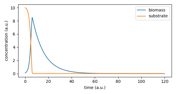
Finally, we visualize the resulting biomass and substrate trajectories.

import matplotlib.pyplot as plt

plt.figure(figsize=(6, 3.2))
plt.plot(sim.t, sim.X[0, :], label="biomass")
plt.plot(sim.t, sim.S[0, :], label="substrate")
plt.xlabel("time (a.u.)")
plt.ylabel("concentration (a.u.)")
plt.legend()
plt.tight_layout()
plt.savefig("crm_simple_example.png")
plt.show()

Here’s what the simulation result look like:

API Documentation

mgrowthctrl.models.crm.model.DType

Either a constant value or a function of time

Type:: The type of the D parameter

alias of float | Callable[[float], float]

mgrowthctrl.models.crm.model.ParamsDict

The type of the param dictionary, with most of its values as ndarrays and the dilution rate given as a float or time-dependent value.

alias of Dict[str, ndarray | float | Callable[[float], float]]

class mgrowthctrl.models.crm.model.CRModelParams( r: ndarray, a: ndarray, b: ndarray, K_ij: ndarray, k: ndarray, S_in: ndarray, D: float | Callable[[float], float], )

Bases: object

Container for CRM parameters.

Dimensions:

n = number of species (consumers)
m = number of resources (metabolites)

r: ndarray: Max growth rates (n, m)

a: ndarray: Resource uptake rates per unit growth (n, m)

b: ndarray: Metabolic byproduct secretion rates (n, m)

K_ij: ndarray: Half-saturation constants (n, m)

k: ndarray: Maintenance/death rates per species (n,)

S_in: ndarray: Inflow resource concentrations (m,)

D: float | Callable[[float], float]: Dilution rate (outflow), either as a constant, or as a function of time

static from_shapes(n: int, m: int, *, init: float = 0.0, D: float = 0.0) → CRModelParams: Initialize parameters with simple constants.

as_dict() → Dict[str, ndarray | float | Callable[[float], float]]: Return params as a dict compatible with crm_fit_backend.

class mgrowthctrl.models.crm.model.CRModel( names: ModelNames, params: CRModelParams, backend: str | ArrayBackend = 'numpy', )

Bases: BaseODEModel

Monod-style Consumer–Resource model using the BaseODEModel.

static from_dict(d: Dict[str, Any], backend: str = 'numpy') → CRModel: Rebuild a CRModel from a dict produced by to_dict().

classmethod from_single_species_data( df, time_col: str, x_col: str, s_cols: List[str], *, K_prefactor: float = 2.0, fit_a: bool = True, n_spline_points: int = 400, r_mask=None, b_mask=None, a_mask=None, backend: str | ArrayBackend = 'numpy', ) → CRModel: Build a single-species CRM with mechanistic initial parameters derived from data. This also attaches the data (_df, _time_col, _x_cols, _s_cols) to the model instance so subsequent .fit() calls don’t need arguments.

set_params(params: CRModelParams) → CRModel: Set internal parameter arrays from a CRModelParams instance.

get_params() → CRModelParams: Return a copy of the current parameters.

compute_rhs(t, X, S): Compute dX/dt, dS/dt given X, S using current parameters.

fit( df: DataFrame, time_col: str | None = None, x_cols: List[str] | None = None, s_cols: List[str] | None = None, method: Literal['least_squares', 'mcmc'] = 'least_squares', *, params0: Dict[str, ndarray | float | Callable[[float], float]] | None = None, lb_factor: float = 0.0, ub_factor: float = 10.0, X0: ndarray | None = None, S0: ndarray | None = None, include_metabolites: bool = True, weight: Literal['median', 'equal'] = 'median', n_time: int = 300, fit_a: bool = True, nsimu: int = 10000, sigma2: float = 12.0, burn: float = 0.8, nsamp: int = 200, seed: int = 1234, ) → CRModel

High-level fit method. The given parameters are passed along to other functions based on the given method. See the documentation of the relevant fit_ methods for details.

Fits the model in place and returns self. Description of the parameters shared by all the “fit” functions:

Parameters:

df – The DataFrame to fit data to
time_col – The name of the time column in df
x_cols – The names of the consumer (X) columns in df
s_cols – The names of the substrate (S) columns in df
method – The fitting method to use
params0 – A dictionary of initial paramater values that will be used to instantiate a CRModelParams instance if no params have been given at construction time.

fit_least_squares( df=None, time_col: str | None = None, x_cols: List[str] | None = None, s_cols: List[str] | None = None, *, params0: Dict[str, ndarray | float | Callable[[float], float]] | None = None, lb_factor: float = 0.0, ub_factor: float = 10.0, X0: ndarray | None = None, S0: ndarray | None = None, include_metabolites: bool = True, weight: Literal['median', 'equal'] = 'median', n_time: int = 300, fit_a: bool = True, )

Mechanistic least-squares fit. All arguments (df, time_col, x_cols, s_cols) default to attached/internal values if None.

A description of the least-squares-specific parameters:

Parameters:

lb_factor – Lower bound factor, multiplied with starting parameters to determine the lower bound of the estimation.
ub_factor – Upper bound factor, multiplied with starting parameters to determine the upper bound of the estimation.
X0 – Initial X values, will be estimated from the data if not given
S0 – Initial S values, will be estimated from the data if not given
include_metabolites – Whether to calculate time-series residuals for metabolites (S) or only for species (X).
weight – Per-species/per-metabolite weighting. If “median”, scales weights based on the median value of the data. If “equal”, does not scale weights.

fit_mcmc( df=None, time_col: str | None = None, x_cols: List[str] | None = None, s_cols: List[str] | None = None, params0: Dict[str, ndarray | float | Callable[[float], float]] | None = None, fit_a: bool = True, nsimu: int = 10000, sigma2: float = 12.0, burn: float = 0.8, nsamp: int = 200, seed: int = 1234, )

Run MCMC parameter estimation. All arguments (df, time_col, x_cols, s_cols) default to attached/internal values if None.

A description of the MCMC-specific parameters:

Parameters:

nsimu – Number of simulations in each chain
sigma2 – Initial observation error
burn – Fraction of samples to drop as burn-in
nsamp – Number of posterior samples to pick
seed – Random seed

simulate( y0: ndarray | torch.Tensor | list | tuple | float | int, t: ndarray | torch.Tensor | list | tuple | float | int, *, log_space: bool = False, method: str | None = None, solver_options: Dict | None = None, ) → SimpleNamespace: A convenience wrapper for BaseODEModel.predict

to_dict() → Dict[str, float | list]: Serialize model to a dict.

References

Levins, R. (1968). Evolution in changing environments: some theoretical explorations (No. 2). Princeton University Press.
MacArthur, R. (1970). Species packing and competitive equilibrium for many species. Theoretical Population Biology, 1(1), 1-11.
Niehaus, L., Boland, I., Liu, M., Chen, K., Fu, D., Henckel, C., … & Momeni, B. (2019). Microbial coexistence through chemical-mediated interactions. Nature Communications, 10(1), 2052.
Butler, S., & O’Dwyer, J. P. (2018). Stability criteria for complex microbial communities. Nature Communications, 9(1), 2970.