Advanced: Diauxic Shift Model
This example is based on Roseburia intestinalis growth data and shows how to implement diauxic-shift behavior as a small extension of the CRModel. The model follows the standard consumer-resource equations, but secondary-substrate uptake is suppressed while glucose is available.
We model the switch using
When glucose is abundant, \(\phi\) is close to zero, so secondary-substrate uptake is nearly switched off. As glucose is depleted, \(\phi\) approaches one and secondary-substrate uptake is switched on.
Custom CRM Class
The example below uses the NumPy backend and overrides only compute_rhs(). All other functionalities are inherited from CRModel.
class DiauxicShiftCRModel(CRModel):
    """CRM with glucose-gated secondary-substrate uptake."""

    def __init__(
        self,
        names,
        params,
        *,
        K_shift,
        glucose_idx,
        secondary_idxs,
        post_glucose_secretion_factors=None,
    ):
        super().__init__(names=names, params=params, backend="numpy")
        self.K_shift = float(K_shift)
        self.glucose_idx = int(glucose_idx)
        self.secondary_idxs = list(secondary_idxs)

        # Fraction of secretion that remains after glucose depletion.
        # Unspecified secondary substrates default to zero.
        self.post_glucose_secretion_factors = {
            int(j): float(v)
            for j, v in (post_glucose_secretion_factors or {}).items()
        }

    def compute_rhs(self, t, X, S):
        X_kin = np.maximum(np.asarray(X, dtype=float), 0.0)
        S_arr = np.asarray(S, dtype=float)
        S_kin = np.maximum(S_arr, 0.0)
        D = self._D_at(t)

        # Low during glucose availability, high after glucose depletion.
        phi = self.K_shift / (self.K_shift + S_kin[self.glucose_idx] + 1e-12)

        # Diauxic shift: suppress secondary-substrate growth rates by phi.
        r_eff = self.r.copy()
        r_eff[:, self.secondary_idxs] *= phi

        # Glucose-dependent byproduct secretion.
        b_eff = self.b.copy()
        for j in self.secondary_idxs:
            residual = self.post_glucose_secretion_factors.get(j, 0.0)
            b_eff[:, j] *= (1.0 - phi) + phi * residual

        monod = S_kin[None, :] / (S_kin[None, :] + self.K_ij + 1e-12)
        growth_terms = r_eff * monod

        growth = growth_terms.sum(axis=1)
        secretion = (b_eff * X_kin[:, None]).sum(axis=0)
        uptake = (self.a * growth_terms * X_kin[:, None]).sum(axis=0)

        dX_dt = (growth - self.k - D) * X_kin
        dS_dt = secretion - uptake + D * (self.S_in - S_arr)
        return dX_dt, dS_dt
Load Data and Build the Model
The parameters are initialized manually; no fitting optimizer is called.
from mgrowthctrl.utils.data import Dataloader

data = Dataloader()
data.load_local_data(
    "examples/datasets/SMGDB00000002/RI_WC.csv",
    x_selector=r"Cells",
    s_selector=[
        "acetate (mM)", "butyrate (mM)", "formate (mM)", "glucose (mM)",
        "lactate (mM)", "pyruvate (mM)", "trehalose (mM)",
    ],
)

s_names = data.S_names
idx = {name: s_names.index(name) for name in s_names}

params = CRModelParams.from_shapes(n=1, m=len(s_names))
params.K_ij[0] = 2.0 * data.df[s_names].max().to_numpy(dtype=float)

model = DiauxicShiftCRModel(
    names=data.names,
    params=params,
    K_shift=0.5,
    glucose_idx=idx["glucose (mM)"],
    secondary_idxs=[
        idx[c] for c in ["acetate (mM)", "lactate (mM)", "butyrate (mM)"]
    ],
    post_glucose_secretion_factors={
        idx["butyrate (mM)"]: 1.5e-2,
    },
)
Parameters that remain zero are inactive. For example, we assume trehalose consumption to be vanishingly small, which is consistent with the underlying data. The post_glucose_secretion_factors argument specifies the fraction of
byproduct secretion that remains after glucose depletion. Here, butyrate keeps a small residual secretion rate, while acetate and lactate secretion vanish after glucose is depleted.
The nonzero entries below specify primary growth on glucose and pyruvate, delayed use of lactate and acetate, and glucose-coupled production of selected byproducts.
p = model.get_params()

p.r[0, idx["glucose (mM)"]] = 0.9
p.a[0, idx["glucose (mM)"]] = 1e-8

p.r[0, idx["pyruvate (mM)"]] = 0.7
p.a[0, idx["pyruvate (mM)"]] = 1e-8

p.r[0, idx["lactate (mM)"]] = 3e-4
p.a[0, idx["lactate (mM)"]] = 1e-6
p.b[0, idx["lactate (mM)"]] = 6e-10

p.r[0, idx["acetate (mM)"]] = 8e-6
p.a[0, idx["acetate (mM)"]] = 1e-5
p.b[0, idx["acetate (mM)"]] = 1.1e-9

p.b[0, idx["butyrate (mM)"]] = 1.8e-9
p.b[0, idx["formate (mM)"]] = 6e-12
p.k[0] = 0.03

model.set_params(p)
Simulation
We will now simulate the model and plot the results.
from mgrowthctrl.utils.plot import plot_data_with_overlay

t_sim = np.linspace(data.start_time, data.end_time, 500)
sim = model.simulate(data.y0, t_sim)

plot_data_with_overlay(
    df=data.df,
    sim=sim,
    overlay="both",
    time_col=data.time_col,
    x_cols=data.X_names,
    s_cols=data.S_names,
    save_prefix="diauxic_shift_plot",
)
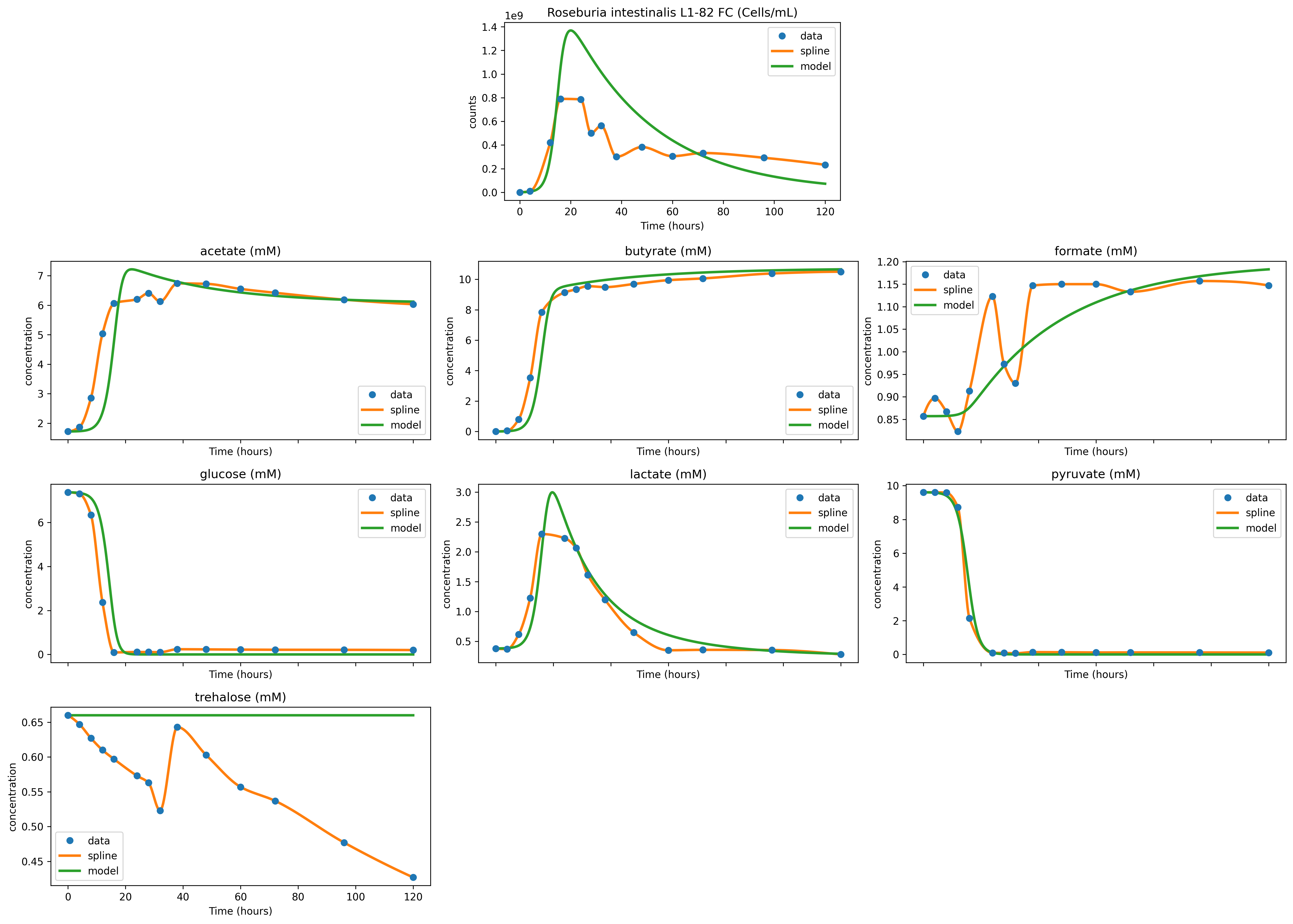
Here’s what the diauxic-shift simulation looks like:
Optional: Parameter Fitting
One can also let the custom model use the inherited fit_least_squares() method.
# Optional: Adjust parameters with the inherited CRM optimizer.
# This updates the model parameters in place.

theta_opt, sim_fit, fit_info = model.fit_least_squares(
     df=data.df,
     time_col=data.time_col,
     x_cols=data.X_names,
     s_cols=data.S_names,
     include_metabolites=True,
     weight="median",
)

print(f"Converged: {fit_info['success']}  residual: {fit_info['cost']:.4g}")