Advanced: Open-Loop Control of Microbiome Dynamics

This tutorial builds on the Get Started example and demonstrates how to steer bacterial concentrations using an open-loop neural ODE controller. For further details on neural ODE–based control, see the references below.

Loading Data

As in the Get Started example, we load experimental time-series data from the BT_WC_export.csv file:

from mgrowthctrl.utils.data import Dataloader

data = Dataloader()
data.load_local_data(
    "examples/datasets/BT_WC_export.csv",
    x_selector=r"BT counts",
)

For further details on the data loader, see the Data Loading section.

Initializing and Fitting a CRM

We first create and fit a CRM to reproduce the output from the Get Started example:

from mgrowthctrl.models.crm.model import CRModel, CRModelParams

# Initialize parameters
params = CRModelParams.from_shapes(n=len(data.X_names), m=len(data.S_names))

# Initialize model with parameters from the data
model = CRModel.from_single_species_data(
    df=data.df,
    time_col=data.time_col,
    x_col=data.X_names[0],  # Note: expects a single species string here
    s_cols=data.S_names,
)

model.fit(
    df=data.df,
    time_col=data.time_col,
    x_cols=data.X_names,
    s_cols=data.S_names,
)

Setup and Train Open-Loop Controller

Since we have fitted the model using the NumPy backend, we need to switch to the PyTorch backend to use automatic differentiation for controller training. This is done by extracting the fitted parameters and reinitializing the model with the PyTorch backend.

params = model.get_params()
model_torch = CRModel(names=data.names, params=params, backend="torch")

We now define a custom loss function that penalizes deviations from a target biomass of \(10^6\) at the final time point, as well as excessive control effort.

import torch
import numpy as np

torch.manual_seed(42)
np.random.seed(42)

def steering_loss(trajectory, controller, model):
    final_biomass = trajectory[-1, 0]
    target_tensor = torch.tensor(1e6, dtype=torch.float32)
    error = (torch.log(final_biomass + 1e-6) - torch.log(target_tensor + 1e-6)) ** 2

    steps = trajectory.shape[0]
    times = torch.linspace(0, controller.total_time, steps, dtype=torch.float32)
    t_norm = (times / controller.total_time).unsqueeze(1)

    U_tensor = controller.net(t_norm)
    cost = 1e-3 * U_tensor.pow(2).mean()

    return error + cost, U_tensor

Next, we initialize an open-loop neural ODE controller.

from torch import nn
from mgrowthctrl.controllers import OpenLoopNeuralController

controller = OpenLoopNeuralController(
    total_time=100,
    n_species=model_torch.n,
    n_resources=model_torch.m,
    s_idx=[2, 4],
    criterion=steering_loss,
    hidden_dims=[5, 5, 5],
    activation=nn.ELU(),
)

We optionally define a logging function to monitor training progress.

def log_fn(model, epoch, loss, U_trajectory, sol_tensor):
    if epoch % 10 == 0:
        actual = sol_tensor[-1, 0].item()
        print(
            f"Epoch {epoch:03d} | Loss: {loss.item():.4f} "
            f"| Target: {1e6:.1e} | Actual: {actual:.1e}"
        )

Finally, we prepare the initial conditions and train the controller.

y0_numpy = data.df[[data.X_names[0]] + data.Y_names].iloc[0].to_numpy(dtype=float)
y0_torch = torch.tensor(y0_numpy, dtype=torch.float32)
t_eval = np.linspace(0, 100, 100)
t_span = (0, 100)

controller.fit(model_torch, y0_torch, t_eval, t_span, epochs=101, lr=1e-2, log_fn=log_fn)

Visualization of Controlled Dynamics

We compare the uncontrolled system dynamics with the controlled trajectory obtained from the trained controller.

uncontrolled_sol = model_torch.solve(
    y0_torch, t_span, t_eval, return_raw_tensors=False
)
controlled_sol = controller.simulate(
    model_torch, y0_torch, t_eval, t_span
)

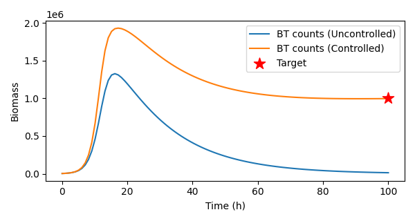
Finally, we visualize the effect of control on the biomass trajectory.

import matplotlib.pyplot as plt

fig, ax = plt.subplots(figsize=(6, 3.2))
ax.plot(
    uncontrolled_sol.t,
    uncontrolled_sol.y[0],
    label=f"{model.names.X[0]} (Uncontrolled)",
)

ax.plot(
    controlled_sol.t,
    controlled_sol.y[0],
    label=f"{model.names.X[0]} (Controlled)",
)
ax.scatter(
    [100],
    [1e6],
    color="red",
    s=150,
    marker="*",
    label="Target",
    zorder=10,
)
ax.set_xlabel("Time (h)")
ax.set_ylabel("Biomass")
ax.legend()
plt.tight_layout()
plt.savefig("open_loop_result.png")
plt.show()

We observe that the controlled dynamics reaches the desired concentration:

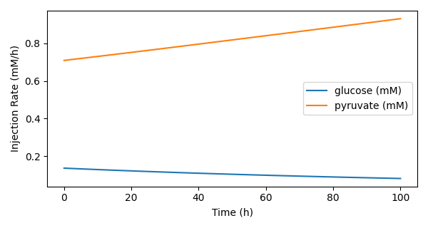
We can also inspect the learned control inputs (injection rates) over time to understand how the controller steers the system toward the target state.

raw_u = controller.get_input_history(t_eval, model_torch).detach()

fig, ax = plt.subplots(figsize=(6, 3.2))
for k, s_idx in enumerate(controller.s_idx):
    ax.plot(
        t_eval,
        raw_u[:, k],
        label=f"{model.names.S[s_idx]}",
    )
ax.set_xlabel("Time (h)")
ax.set_ylabel("Injection Rate (mM/h)")
ax.legend(loc=5)
plt.tight_layout()
plt.savefig("open_loop_control_inputs.png")
plt.show()

Here’s what the result looks like:

References

• Asikis, T., Böttcher, L., & Antulov-Fantulin, N. (2022). Neural ordinary differential equation control of dynamics on graphs. Physical Review Research, 4(1), 013221.

• Böttcher, L., Antulov-Fantulin, N., & Asikis, T. (2022). AI Pontryagin or how artificial neural networks learn to control dynamical systems. Nature Communications, 13(1), 333.

• Böttcher, L., & Asikis, T. (2022). Near-optimal control of dynamical systems with neural ordinary differential equations. Machine Learning: Science and Technology, 3(4), 045004.

• Böttcher, L. (2026). Control of dynamical systems with neural networks. Nonlinear Dynamics, 114(2), 79.